
Open Access Journal of Agriculture Research
Export, Foreign Direct Investment (FDI) and Economic Growth in Ethiopia: VAR Analysis
Ahmed Kasim Dube1 and Burhan Özkan2*
1PhD student at Department of Agricultural Economics, Faculty of Agriculture, Akdeniz University, Antalya, Turkey
2*Department of Agricultural Economics, Faculty of Agriculture, Akdeniz University, Antalya, Turkey
*Corresponding author: Burhan Ozkan, Department of Agricultural Economics, Faculty of Agriculture, Akdeniz University, Antalya, Turkey, Tel: +902423102475, Fax: +902422274567.
Citation: Ozkan B, Dube AK (2018) Export, Foreign Direct Investment (FDI) and Economic Growth in Ethiopia: VAR Analysis. Open Acc J Agri Res: OAJAR-1000111.
Received Date: 26 October, 2018; Accepted Date: 26 November, 2018; Published Date: 06 December, 2018
1. Abstract
The objectives of this paper was to examine long run dynamic relationship between FDI, export and economic growth in Ethiopia using long run data from 1970-2016. Vector autoregressive model was implemented to achieve the objective. The lag selection criteria applied to the VAR model revealed VAR (1) model was an optimal model for the study. The results of Johansen Cointegration technique indicated that there is no cointegration between the series. However, the Granger Causality/Block Exogeneity Wald Tests statistics showed that there is unidirectional causal flow from FDI and export to GDP. There is no Granger causality from GDP to other series. This result was supported by the impulse response relationship and variance decomposition analysis. The result showed that the shock to GDP has positive effect on its values. But, it had zero effect on both export and FDI. There was significant and positive impulse response relationship from export to GDP throughout the period. About 80% of variation in GDP was caused by export. Similarly, the Granger causality from FDI to GDP was also significant. Thus, the evidence suggests that Ethiopia should emphasize the export-led growth strategy in addition providing good environments to attract more capital investments with enhanced technology and competitive industrial productions for exports.
2. Keywords: Export; FDI; Economic growth; Vector autoregressive regression
3. Introduction
Examination of the casual relationship between foreign direct investment (FDI), export, and economic growth has attracted the attention of researchers and continues to be of a crucial interest among policy makers in both developing and developed countries. This was motivated by the role that foreign direct investment and export have played in many economies of the world. However, depending on the period under consideration and the econometric methods applied, varied causal relationships were obtained between these series in different countries of the world [1].
Several studies were undertaken to examine the causal relationship between FDI and economic growth. This was motivated by the role that foreign direct investment has played in many economies of the world. There was also widespread belief among policy makers that foreign direct investment enhances the productivity of host countries and promotes development [2]. Frank and Mei-chu (2006) [3] using time series and panel data from 1986 to 2004 examined the granger causality relationship between GDP, export and FDI among eight rapidly growing east and Southeast Asian economies. The results revealed that FDI has unidirectional effects on GDP directly and indirectly through export. Similar results were found by Odongo (2012) [4] who used multivariate vector autoregressive model (VAR) and investigated the impact of foreign direct investment (FDI) on economic growth of Uganda for the periods between 1970 and 2010. The finding of the study indicated that foreign direct investments are of great importance in stimulating economic growth in Uganda. Foreign direct investment had affected economic growth in three different channels which includes direct transmission from FDI to GDP growth, indirectly through domestic investments by multiplier process, and through exports by which it yields export led growth.
The causal relationship is not always from FDI to economic growth. Bianca (2012) [5] using VAR examined the causal relationship between FDI and Economic growth in Romania between 1991-2009. FDI was obtained not initiating economic growth while economic growth was an important factor in terms of attracting FDI in Romania. Similar result was obtained by Ingo (2015) [6] in his study in Namibia made by applying the autoregressive Distributed Lag (ARDL) approach to quarterly data for the period from 1980: Q1 to 2013: Q4. The results from the study indicated that economic growth was explained by itself and FDI does not have a role to play in explaining economic growth both in the short run and long run. However, an empirical works undertaken by [1] for Romania revealed different result. They used vector error correction model (VECM) to analyse quarterly data for the period from 2005-2014. Their finding indicated that there was a positive significant bidirectional relationship between FDI and GDP. More than 50% of fluctuation in FDI was caused by shocks in GDP. Romero (2015) [7] in his study also obtained that there was bidirectional causality between FDI and GDP.
Several empirical works had also examined the causal relationship between FDI and export. Like the previous causal relationship, there was also no unanimity in the direction whether FDI causes exports or exports cause FDI. Martin (2010) [8] examined the dynamics of export and outward foreign direct investment flows in Spain using time series data from 1993-2008. The result of multivariate co-integrated model (VECM) indicated that there was a positive Granger (causality) relationship running from FDI to export of goods (stronger) and to export of services (weaker) in the long run. In the short run, however, only exports of goods are affected (positively) by FDIs. The relationship between export and FDI are either direct or indirect. Similarly, the work of Romero (2015) [7] in Mexico showed that FDI and export are either directly or indirectly related. In the empirical work of Nguyen (2011) [9] for Korea and Malaysia, bidirectional relationship was obtained in Malaysia while no causal relationship was obtained in Korea between FDI and export. They attributed these differences to different economic policy followed by the two countries. That is, although both countries implemented policies of export-orientated industrialization, the Malaysian government promoted FDI as a tool of industrialization, while the Korea government built an “integrated national economy” using industrial structures and minimizing the role of FDI.
The other important relationship is the causality that dictates either export-led-growth or growth-led-exports. Uni-directional causality between export and economic growth was obtained for Ethiopia suggesting export-led growth strategy [10,11]. However, empirical work by Hussain (2014) [12] for Pakistan showed that even though relationship exists between economic growth (GDP) and export, worthy of note is that causality runs from economic growth to export. These indicate that there is no agreement among researchers as to whether the causality is from export to economic growth or vice versa.
Therefore, the three types of causal relationship between FDI, export and economic growth mentioned above varies depending on the analyzed period, the countries that are studied and the econometric methods applied. There is no clear causality between these variables. Different empirical works either confirmed unidirectional or bidirectional causality relationships, while others indicated absence of any type of causality [13]. In Ethiopia, the study so far undertaken focused either only on causal link between economic growth and export [11, 14-16] or on FDI and economic growth [17,18]. But as it is indicated in the previous paragraphs, there is possibility of causal flow between these three economic variables. Without understanding the direction of the relationships between these variables, it is not possible to draw important lessons for policy making purposes in an effort to pursue more effective policies that promote economic growth. Therefore, the objective of this paper was to find the causality relationship between FDI, export and economic growth in Ethiopia.
4. Methodology
4.1. Description of data
The purpose of this study was to examine the dynamic relationship between real economic growth as measured by real GDP and selected macroeconomic variables including export and FDI. They were sourced from UNCTAD data base, World Bank open data base and National bank of Ethiopia annual report (NB, 2016/17) [19]. These annual data covering the period from 1970 to 2016 were expressed in natural logarithms. Consequently, LNGDP is the logarithm of real GDP, LNEXPORT is the logarithm of real exports and LNFDI is the logarithm of real foreign direct investment. All the variables are expressed in millions of US dollars before taking logs. The following figure describes our three series including LNDGP (Figure 1), LNEXPORT (Figure 2) and LNFDI (Figure 3) for Ethiopia.
4.2. Building the vector autoregressive model (VAR)
The VAR model developed by Sims (1980) [20] was used by many researchers to examine the dynamic relationships between two (or more) time series variables in different part of the world. In this study also VAR model was used to study the causal relationship between export, FDI and economic growth in Ethiopia. Following Lütkephol (2005) [21] the general VAR (p) model is described as follows:

From this general VAR (p) model, we developed a VAR (1) model for DLNGDP, DLNFDI and DLNEXPORT. The scalar notation of VAR (1) model was described as follows:
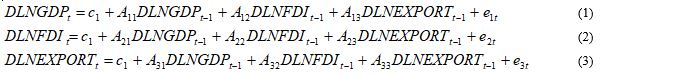
As shown in the above VAR (1) model, all variables were considered as endogenous variable. Consequently, three equations were developed with similar regressors, which are the lagged values of DLNGDP, DLNFDI and DLNEXPORT. ci and Aij are the intercept terms and regression coefficient respectively. eit represents error in prediction of each outcome at time t. The equations were solved using ordinary least squares (OLS) estimation. To check consistency of parameters, diagnosis test including autocorrelation test, heteroscedasticity and normality test were applied to the estimated VAR model.
4.3. Tools for testing unit root of time series
There are a variety of powerful tools for testing a series (or the first or second difference of the series) for the presence of a unit root. But, in this paper Augmented Dickey-Fuller (1979) [22] and Phillips-Perron (1988) [23] test were used to test the stationarity of data. The test was conducted for both level and differenced data using model only with intercept and model with intercept and trend (VAR Ethiopia).
4.4. Cointegration test
Co-integration is a powerful way of detecting the presence long run relationship or steady state equilibrium between variables [24]. Different co-integration techniques that were developed to determine the long run relationship between time series includes [25], Autoregressive Distributed Lag (ARDL) co-integration technique or bound test of co-integration [26-28]. Among these techniques, a Johansen (1988) [27] Cointegration technique was used in this study. In the absence of cointegration, long run relationship between variables can be studied by using VAR.
4.5. Granger causality model
The concept of causality defined by Granger (1969) has become quite popular in recent years. The idea is that if zt can be predicted more efficiently by taken into account information in xtprocess in addition to all other information in the universe, then xt is Granger-causal for zt [21].
The Granger causality will be tested by applying Granger causality/Block erogeneity Wald statistics test. This test will helps us to know whether the lags of one variable can Granger cause any other variables in the VAR system. Accordingly, the null hypothesis stating all lag of a variable can be excluded from the model is tested against alternative hypothesis in which all lags of a variable cannot be excluded. Rejection of the null is an indication of causality between variables [29].
4.6. The impulse-response function
The results of Granger cause cannot tell us the direction and the size of Granger cause. These are obtained by analyzing the impulse-response function and the variance decomposition. An impulse response function was used to trace the effect of a one-time shock to one of the innovations on current and future values of the endogenous variables through the dynamic lag structure of the VAR model estimation. According to Lütkephol (2005) [21], impulse responses can be computed easily from the structural form parameters. Rewriting the VAR in levels form as:

4.7. Variance decomposition
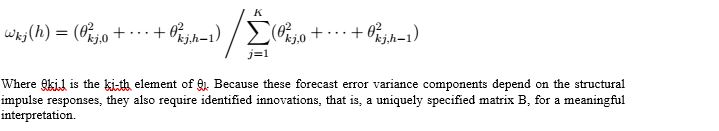
Forecast random error variance decompositions are alternative tools for analyzing the dynamic interactions between the variables of a VAR model [21]. It tells us by how much a given variable changes due to its own shocks and the shocks of other variables. If a variable is not affected by random effect of any of the variables in the VAR system then the variable is said to be exogenous. If however, the random error of any variable affects the forecast error of variable at all forecast period, then the variable is said to be endogenous. Thus, forecast random error variance decomposition defines the relative importance of each random innovation in affecting the variables in the VAR [29]. Denoting by wkj(h) the percentage contribution of variable j to the h-step forecast error variance of variable k, it can be shown that [21]:
5. Estimation and Discussion of Results
5.1. Unit root test results
To mitigate fluctuation, the real values of all economic variables were transformed into logarithmic values. According to results presented in (Table 1), the test results of both Augmented Dickey-Fuller (ADF) and Philips-Perron showed that there is no stationarity in the level data both in only intercept and with both intercept and time trend model. Their absolute values are less than the absolute value of 5 percent critical value of - 2.927. Thus, they have a unit root and we continue to test the unit root of their first difference. In this case (Table 2), since their absolute values are higher than the absolute value of 5 percent critical values of -3.19, we can reject the null hypothesis of non-stationary at a 0.05 level. Thus, we can conclude that the series are integrated of order 1 (i.e., I (1)).
5.2. Determining lag order
According Lütkephol (2005) [21], using too few lags can results in auto correlated errors whereas using too many lags results in over fitting of the VAR model. Consequently, the choice of the optimal lag-length was made by minimizing the sequential modified LR test statistic (LR), Final prediction error (FPE), Akaike Information Criteria (AIC) and Schwarz Bastian Information Criteria (BIC). According to results presented in (Table 3), all the five criteria (LR, FPE, AIC, SC and HQ) recommend a VAR model with lag equal to 1. Consequently, the joint optimal lag length of order one (VAR (1)) was estimated.
5.3. Co-integration test
Testing the existence of long-term relationship between the dependent and the explanatory variables in a multivariate framework necessitates determination of the degree of co-integration between vectors. The determination of the number of co-integrating vectors is usually based on the method of two likelihood ratio (LR) test statistics; the trace test and the maximum eigen value test. In this study the test was made using both tests.
Consequently, testing the hypothesis that the variables are not co-integrated (r=0) against the alternative of one or more co-integrating vectors (r>0), was tested by looking at the value of λTRACE or λMAX. Column 3 of the first part of Table 4 presents the trace values corresponding to each number of the cointegrating vector: λTRACE (0) = 25.345, λTRACE (1) = 12.594, and λTRACE(2) = 4.779. The corresponding critical values are 35.193, 20,262 and 9.165 respectively. Since the value of λTRACE is less the critical values for every number of co-integration indicated in (Table 4), we fail to reject the null hypothesis. Consequently, the λ TRACE test statistcis indicates the absence of cointegration between GDP, export and FDI. Similar results were obtained by using the maximum eigen value statistics. Results of λMAX (0), λMAX(1), and λMAX(2) are presented in Column 3 of the second part of Table 4. These values: λMAX (0)= 12.752, λMAX (1)= 7.815 , and λMAX (2)= 4.779 are all less than their 5% critical vales of 22.299, 15.892 and 9.165 respectively. This test statistics also fails to reject the null hypothesis. Therefore, using both trace and maximum eigen values we can conclude that there is no co-integration between GDP, export and FDI. The decision of the choice between VECM and VAR could also be made easily using these information. VECM cannot be used to study the relationship between GDP, export and FDI. But, we can use VAR to study their relationship. Consequently, our model follows VAR (1) model. Thus, VAR (1) is fitted to the stationary differenced data and diagnostic tests with respect to the residuals were tested.
5.4. Vector autoregression
(Table 5) presents the estimation results of VAR (1) model. It was estimated to examine dependency of LNGDP, LNEXPORT and LNFDI on their own past and the past values of the other variables. Stability test of VAR (1) model was also tested. According results presented in (Table 6), VAR satisfies the stability condition.
5.5. Diagnostic checking
5.5.1. Testing for residual autocorrelation
In time series models, autocorrelation of the residual values is used to determine the goodness of fit of the model. Autocorrelation of the residuals indicates that there is information that has not been accounted for in the model. Consequently, the null hypothesis which states there is no residual autocorrelation against the alternative hypothesis which claims the existence of residual autocorrelation was tested by using the Lagrange Multiplier (LM) test which is the standard tool for checking residual autocorrelation in VAR models. Results presented in (Table 7) shows that the LM-statistics values for the lag order of 1, 2 provides evidence for acceptance of null hypothesis of no autocorrelation at each lag. Thus, there is no problem of residual autocorrelations in VAR (1) model.
5.5.2. Heteroscedasticity test
The other important diagnostic test in VAR model test is the test of heteroscedasticity test. Accordingly, the null hypothesis stating there is heteroscedasticity was tested against the alternative hypothesis providing evidence for the presence of homoscedasticity. The result presented in (Table 8) provides enough evidence for the rejection of our null hypothesis. Therefore, absence of the problem of heteroscedasticity in our VAR model is an indication for the goodness of our model.
5.5.3. Normality test
According to results presented in (Table 9), we cannot reject the hypothesis of normality properties. This is because, P-values of 0.0162, 0.2443 and 0.0249 for skewness, kurtosis and the Jarque-Bera test are all greater than 0.01 respectively. This provides some evidence for the hypothesis that residuals from our VAR model have a normal distribution.
5.6. Granger Causality
(Table 10) presents the results from the Granger Causality/Block Exogeneity Wald Tests and includes three parts. The first part reports the result of testing that shows whether we can exclude each variable from the equation of DLNGDP. Table 10 includes four columns each specifying lists of the variables that will be excluded from the equation, the value of the Chi-square test, degrees of freedom and P-value respectively. The last row in each part of the table reports the joint statistics of the variables excluded from the equation.
Results corresponding to the DLNGDP equation shows that the Chi-squares for DLNFDI,
and DLNEXPORT are respectively 4.934086 and 9.058188. The p value of both of them is less than 5% indicating significance in granger cause of both variables. Thus, we reject the null hypothesis for both variables and conclude that there is causality from DLNFDI and DLNEXPORT to DLNGDP. This is confirmed by the fact that the joint Chi-square is significant. Thus, in both cases, we reject the null hypothesis to exclude variables from the equation of DLNGDP and came to conclusion of existence of causality between variables.
In the second part of Table 10, DLNFDI equation is presented with respective Chi-squares values of DLNGDP and DLNEXPORT. In this case we test the null hypothesis that there is no granger causality from DLNGDP and DLNEXPORT to DLNFDI. The Chi-square of DLNGDP and DLNEXPORT is 0.604167 and 0.269054 respectively. The corresponding p value of both variables is greater than 5%. This indicates that individually there is no granger cause from DLNGDP and DLNEXPORT to DLNFDI. The joint effect Chi-square value is (1.170263) also not significant (P>0.05). Therefore, we can conclude that there is no Granger causality from both DLNGDP and DLNEXPORT to DLNFDI.
The final section of Table 10 is about Granger causality flow from DLNGDP and DLNFDI to DLNEXPORT. The chi-square value is 0.932625 and 0.880689 for DLNGDP and DLNFDI respectively. Comparing their corresponding p-values with 5% indicates that both variables are individually not the granger cause of DLNEXPORT. Similarly, the joint effect chi-square value of both variables is not significant. This indicates that individually and jointly, there is no Granger causality from DLNGDP and DLNFDI to DLNEXPORT.
5.7. The impulse response relationship
As it is mentioned in the previous sections, VAR is an important tool to analyze the long run relationship between economic variables. Important elements of VAR estimation used to study long run relationship between variables including impulse response relationship and variance decomposition analysis were estimated to see how the shock in one of the variables is going to affect the long run values of the other variables.
Results presented in (Figure 4-6) shows how the shock to DLNGDP is going to affect the long run values of DLNGDP, DLNFDI and DLNEXPORT. In figure 4, it could be seen that the shock to DLNGDP has positive effect on its values. But, this positive effect will soon disappear after five year which results zero effect of shock to DLNGDP to its own values. In the case of export and DLNFDI, the shock to DLNGDP has zero effect to both DLNEXPORT and DLNFDI. This results to similar to the Granger-cause results presented in the previous section in which it was revealed DLNGDP is not the Granger cause of both DLNEXPORT and DLNFDI. Therefore, it can be concluded from both the Granger and impulse response function that shocks to DLNGDP do not affect the long run values of both DLNFDI and DLNEXPORT.
The effects of shocks to DLNEXPORT to DLNGDP, DLNFDI and DLNEXPORT were presented in (Figure 10-12). The effect of the shocks to DLNGDP was positive throughout the period. This is similar with the results obtained in Granger Causality/Block Exogeneity Wald Tests. There was significant and positive Granger cause from DLNEXPORT to DLNGDP. However, the effect of the shocks to DLNFDI was zero throughout the period. Granger Causality/Block Exogeneity Wald Tests also showed the same results. The shocks to DLNEXPORT had also positive effects in the case of the long run value of DLNEXPORT. But the effect had disappeared in the final years.
5.8. Variance Decomposition
(Table 11) reports the variance decomposition of each endogenous variable used for the estimation of VAR (1) including DLNGDP, DLNFDI and DLNEXPORT respectively. In addition to the standard error of the sample set, the variance proportion of the shock to each variable in each time period were presented in the third column to column five under three sections.
According results presented in the first section of Table 11, the fluctuations of DLNGDP are explained mainly by DLNGDP shocks and DLNEXPORT shocks, in the long run. In the first year 100% of shocks came from DLNGDP shock. Its proportion in the variance of DLNGDP decreases over time and reaches 17.89% in the last year. DLNEXPORT shock accounts for 0% in the first year in variance decomposition of DLNGDP. However, its proportion increases over time and reaches 80% in the last year. In the case of variance decomposition of DLNEXPORT, DLNEXPORT shock which is assumed to account for the whole variance of DLNEXPORT in the first year, continuo dominating in the following years. The effect of shocks from both DLNGDP and DLNFDI are almost insignificant in DLNEXPORT variance decomposition analysis. Finally, the variance decomposition of DLNFDI also revealed that the shock of DLNFDI dominates the variation right from the beginning up to the end of the period. The shocks from both DLNGDP and DLNEXPORT were very low. Therefore, the evidence suggests that FDI shock is the sole factor explaining DLNFDI variability. DLNFDI shock accounts for about 99.99% in the first year. This high proportion continuo dominating the whole period until it finally decline to 86.8% in the last year.
6. Conclusion
In this paper the long run dynamic relationship between foreign direct investment (FDI), export, and economic growth of Ethiopia was examined using long run data from 1970-2016. This was motivated by the role that foreign direct investment and export have played in many economies of the world. However, without understanding the direction of the relationships between these variables, it is not possible to draw important lessons for policy making purposes in an effort to pursue more effective policies that promote economic growth. Consequently, the VAR model developed by [20] was applied to export, FDI and economic growth in Ethiopia to examine their dynamic relationships. The lag selection criteria applied to the VAR model revealed VAR (1) is an optimal model for the study. The results of Johansen (1988) [27] Cointegration technique indicated absence of long run cointegration between the series. As a result, the long run relationship between the series was studied by estimating VAR (1). The diagnostic tests and the stability test results show VAR (1) model is good model to study the relationship between FDI, export and GDP. The Granger Causality/Block Exogeneity Wald Tests statistics showed that there is unidirectional causal flow from FDI and export to GDP. That is, there is no Granger causality from GDP to other series. This result was supported by the impulse response relationship and variance decomposition analysis estimated to see how the shock in one of the variables is going to affect the long run values of the other variables. The result showed that the shock to GDP has positive effect on its values. But, in the case of export and FDI, the shock to GDP has zero effect to both export and FDI. In the case of FDI, the effect of shocks to FDI was positive for few years which disappeared soon. However, this result is opposite to Granger Causality/Block Exogeneity Wald Tests in the case of GDP. The effect of the shocks to export on GDP was positive throughout the period. This is similar with the results obtained in Granger Causality/Block Exogeneity Wald Tests. There was significant and positive Granger cause from export to GDP. However, the effect of the shocks to export on FDI was low at the beginning but started increasing in the last years of the period. The shocks to export had also positive effects in the case of the long run value of its value. Similar results were revealed by the variance decomposition analysis. Thus, the evidence suggests that Ethiopia should emphasize the export-led growth strategy in addition providing good environments to attract more capital investments with enhanced technology and competitive industrial productions for exports.
Figure 1: LNGDP
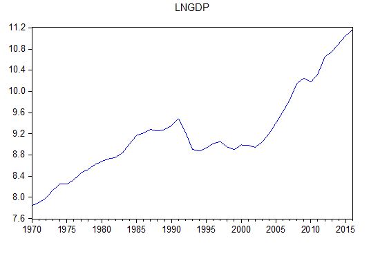
Figure 2: LNEXPORT
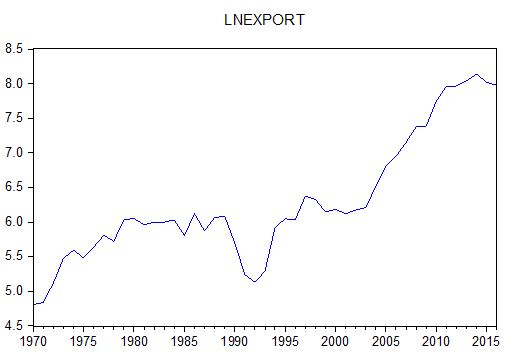
Figure 3: LNFDI
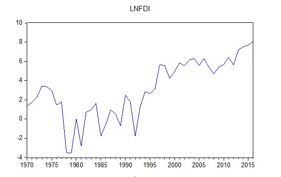
Table 1: Results of ADF and PP level data test statistics.
|
Variables |
ADF test statistics
|
PP test |
||
|
Intercept |
Trend and intercept |
Intercept |
Trend and intercept |
|
|
Lngdp |
0.650280 |
-1.231464 |
0.576170 |
-0.665776 |
|
Lnexport |
-0.496062 |
-1.387676 |
-0.627633 |
-1.617360 |
|
Lnfdi |
-0.454328 |
-3.190757 |
-1.308548 |
-3.082962 |
|
Source: Own computation, critical value at 5% : 2.9 |
||||
Table 2: First difference ADF and PP test statistics results.
|
Variables |
ADF first difference test statistics
|
PP first difference test statistics
|
||
|
Intercept |
Trend and intercept |
Intercept |
Trend and intercept |
|
|
lngdp |
-2.402339 |
-4.379273 |
-3.666488 |
-3.753592 |
|
lnexport |
-5.431495 |
-5.368022 |
-5.438389 |
-5.368022 |
|
Lnfdi |
-7.084626 |
-7.172134 |
-8.807796 |
-8.674488 |
|
Source: Own computation, Critical value at 5%:-3.19 |
||||
Table 3: VAR Lag Order Selection Criteria.
|
Lag |
LogL |
LR |
FPE |
AIC |
SC |
HQ |
|
0 |
-128.8667 |
NA |
0.080510 |
5.994077 |
6.234965 |
6.083877 |
|
1 |
-24.95777 |
184.7270* |
0.001189* |
1.775901* |
2.378122* |
2.000403* |
|
2 |
-19.26107 |
9.367899 |
0.001389 |
1.922714 |
2.886268 |
2.281917 |
|
Source: Own computation, using Eviews 9.0 |
||||||
Table 4: Johansen Cointegration Test with Optimal Lag Length of One.
|
Unrestricted Cointegration Rank Test (Trace) |
||||
|
Hypothesized |
|
Trace |
0.05 |
|
|
No. of CE(s) |
Eigen value |
Statistic |
Critical Value |
Prob.** |
|
None |
0.247 |
25.345 |
35.193 |
0.380 |
|
At most 1 |
0.159 |
12.594 |
20.262 |
0.397 |
|
At most 2 |
0.100 |
4.779s |
9.165 |
0.309 |
|
Trace test indicates no cointegration at the 0.05 level |
||||
|
* denotes rejection of the hypothesis at the 0.05 level |
||||
|
**MacKinnon-Haug-Michelis (1999) p-values |
||||
|
Unrestricted Cointegration Rank Test (Maximum Eigen value) |
||||
|
Hypothesized |
|
Max-Eigen |
0.05 |
|
|
No. of CE(s) |
Eigenvalue |
Statistic |
Critical Value |
Prob.** |
|
None |
0.246764 |
12.752 |
22.299 |
0.5810 |
|
At most 1 |
0.159418 |
7.815 |
15.892 |
0.5700 |
|
At most 2 |
0.100751 |
4.779 |
9.165 |
0.3085 |
|
Max-eigenvalue test indicates no cointegration at the 0.05 level |
||||
|
* denotes rejection of the hypothesis at the 0.05 level |
||||
|
**MacKinnon-Haug-Michelis (1999) p-values |
||||
|
Source: Own computation |
||||
Table 5: Vector Autoregression Estimates.
|
Standard errors in ( ) & t-statistics in [ ] |
|||
|
|
DLNGDP |
DLNFDI |
DLNEXPORT |
|
DLNGDP(-1) |
0.563197 |
-5.044434 |
2.673177 |
|
|
[ 3.94951] |
[-2.22128] |
[ 0.96572] |
|
DLNFDI(-1) |
0.007186 |
-0.41245 |
0.168408 |
|
|
(0.00924) |
(0.14723) |
(0.17945) |
|
|
[ 0.77728] |
[-2.80146] |
[ 0.93845] |
|
DLNEXPORT(-1) |
-0.004646 |
-0.429306 |
-0.116972 |
|
|
(0.00896) |
(0.14264) |
(0.17386) |
|
|
[-0.51870] |
[-3.00968] |
[-0.67277] |
|
C |
0.017335 |
0.009198 |
-0.312559 |
|
|
(0.03539) |
(0.56368) |
(0.68706) |
|
|
[ 0.48975] |
[ 0.01632] |
[-0.45492] |
|
@TREND |
0.000469 |
0.021219 |
0.008391 |
|
|
(0.00151) |
(0.02399) |
(0.02924) |
|
|
[ 0.31109] |
[ 0.88457] |
[ 0.28697] |
|
R-squared |
0.340520 |
0.340992 |
0.078133 |
|
Adj. R-squared |
0.260584 |
0.261113 |
-0.033609 |
|
Sum sq. resids |
0.337606 |
85.62375 |
127.2109 |
|
S.E. equation |
0.101146 |
1.610795 |
1.963384 |
|
F-statistic |
4.259865 |
4.268825 |
0.699228 |
|
Log likelihood |
35.82612 |
-69.35482 |
-76.87661 |
|
Akaike AIC |
-1.622427 |
3.913411 |
4.309295 |
|
Schwarz SC |
-1.406955 |
4.128883 |
4.524767 |
|
Mean dependent |
0.061641 |
0.096310 |
0.034578 |
|
S.D. dependent |
0.117626 |
1.873920 |
1.931200 |
|
Determinant resid covariance (dof adj.) |
0.089990 |
|
|
|
Determinant resid covariance |
0.058937 |
|
|
|
Log likelihood |
-107.9645 |
|
|
|
Akaike information criterion |
6.471814 |
|
|
|
Schwarz criterion |
7.118230 |
|
|
Source: Own computation
Table 6: Roots of Characteristic Polynomial.
|
Endogenous variables: LNGDP LNFDI LNEXPORT |
|
|
Exogenous variables: C @TREND |
|
|
|
|
|
|
|
|
Root |
Modulus |
|
|
|
|
|
|
|
0.904532 - 0.158730i |
0.918353 |
|
0.904532 + 0.158730i |
0.918353 |
|
0.580373 |
0.580373 |
|
|
|
|
|
|
|
No root lies outside the unit circle. |
|
|
VAR satisfies the stability condition. |
|
Source: Own computation
Table 7: VAR Residual Serial Correlation LM Tests
|
VAR Residual Serial Correlation LM Tests |
||
|
Null Hypothesis: no serial correlation at lag order h |
||
|
|
|
|
|
|
|
|
|
Lags |
LM-Stat |
Prob |
|
|
|
|
|
|
|
|
|
1 |
9.465739 |
0.3954 |
|
2 |
5.546117 |
0.7843 |
|
|
|
|
|
|
|
|
|
Probs from chi-square with 9 df. |
||
Source: Own computation
Table 8: VAR Residual Heteroskedasticity Tests: No Cross Terms (only levels and squares).
|
|
|
|
|
|
|
|
|
|
|
|
|
|
|
|
|
|
|
|
|
|
Joint test: |
|
|
|
|
|
|
|
|
|
|
|
|
|
|
|
|
|
|
|
|
Chi-sq |
Df |
Prob. |
|
|
|
|
|
|
|
|
|
|
|
|
|
|
|
|
|
|
59.02705 |
48 |
0.1322 |
|
|
|
|
|
|
|
|
|
|
|
|
|
|
|
|
|
|
|
|
|
|
|
|
|
Individual components: |
|
|
|
||
|
|
|
|
|
|
|
|
|
|
|
|
|
|
|
Dependent |
R-squared |
F(8,29) |
Prob. |
Chi-sq(8) |
Prob. |
|
|
|
|
|
|
|
|
|
|
|
|
|
|
|
res1*res1 |
0.138730 |
0.583902 |
0.7827 |
5.271751 |
0.7282 |
|
res2*res2 |
0.275451 |
1.378113 |
0.2473 |
10.46714 |
0.2338 |
|
res3*res3 |
0.309817 |
1.627230 |
0.1602 |
11.77305 |
0.1616 |
|
res2*res1 |
0.197504 |
0.892158 |
0.5354 |
7.505163 |
0.4832 |
|
res3*res1 |
0.114167 |
0.467195 |
0.8690 |
4.338359 |
0.8254 |
|
res3*res2 |
0.220921 |
1.027929 |
0.4380 |
8.394994 |
0.3959 |
|
|
|
|
|
|
|
|
|
|
|
|
|
|
Source: Source: Own computation
Table 9: VAR Residual Normality Tests.
|
Orthogonalization: Cholesky (Lutkepohl) |
|
|||
|
Null Hypothesis: residuals are multivariate normal |
|
|||
|
|
|
|
|
|
|
|
|
|
|
|
|
|
|
|
|
|
|
Component |
Skewness |
Chi-sq |
df |
Prob. |
|
|
|
|
|
|
|
|
|
|
|
|
|
1 |
-0.289313 |
0.641715 |
1 |
0.4231 |
|
2 |
-1.063073 |
8.664286 |
1 |
0.0032 |
|
3 |
-0.358949 |
0.987805 |
1 |
0.3203 |
|
|
|
|
|
|
|
|
|
|
|
|
|
Joint |
|
10.29381 |
3 |
0.0162 |
|
|
|
|
|
|
|
|
|
|
|
|
|
|
|
|
|
|
|
Component |
Kurtosis |
Chi-sq |
df |
Prob. |
|
|
|
|
|
|
|
|
|
|
|
|
|
1 |
3.040179 |
0.003094 |
1 |
0.9556 |
|
2 |
4.179624 |
2.667066 |
1 |
0.1024 |
|
3 |
3.882689 |
1.493352 |
1 |
0.2217 |
|
|
|
|
|
|
|
|
|
|
|
|
|
Joint |
|
4.163512 |
3 |
0.2443 |
|
|
|
|
|
|
|
|
|
|
|
|
|
|
|
|
|
|
|
Component |
Jarque-Bera |
Df |
Prob. |
|
|
|
|
|
|
|
|
|
|
|
|
|
|
1 |
0.644810 |
2 |
0.7244 |
|
|
2 |
11.33135 |
2 |
0.0035 |
|
|
3 |
2.481157 |
2 |
0.2892 |
|
|
|
|
|
|
|
|
|
|
|
|
|
|
Joint |
14.45732 |
6 |
0.0249 |
|
|
|
|
|
|
|
|
|
|
|
|
|
Source: Own computation
Table 10: VAR Granger Causality/Block Exogeneity Wald Tests.
|
|
|
|
|
|
|
|
|
|
|
|
|
|
|
|
Dependent variable: DLNGDP |
|
||
|
|
|
|
|
|
|
|
|
|
|
Excluded |
Chi-sq |
Df |
Prob. |
|
|
|
|
|
|
|
|
|
|
|
DLNFDI |
4.934086 |
1 |
0.0263 |
|
DLNEXPORT |
9.058188 |
1 |
0.0026 |
|
|
|
|
|
|
|
|
|
|
|
All |
13.13150 |
2 |
0.0014 |
|
|
|
|
|
|
|
|
|
|
|
|
|
|
|
|
Dependent variable: DLNFDI |
|
||
|
|
|
|
|
|
|
|
|
|
|
Excluded |
Chi-sq |
Df |
Prob. |
|
|
|
|
|
|
|
|
|
|
|
DLNGDP |
0.604167 |
1 |
0.4370 |
|
DLNEXPORT |
0.269054 |
1 |
0.6040 |
|
|
|
|
|
|
|
|
|
|
|
All |
1.170263 |
2 |
0.5570 |
|
|
|
|
|
|
|
|
|
|
|
|
|
|
|
|
Dependent variable: DLNEXPORT |
|
||
|
|
|
|
|
|
|
|
|
|
|
Excluded |
Chi-sq |
Df |
Prob. |
|
|
|
|
|
|
|
|
|
|
|
DLNGDP |
0.932625 |
1 |
0.3342 |
|
DLNFDI |
0.880689 |
1 |
0.3480 |
|
|
|
|
|
|
|
|
|
|
|
All |
1.670292 |
2 |
0.4338 |
|
|
|
|
|
|
|
|
|
|
Source: Own computation
Table 11: Variance decomposition.
|
|
|
|
|
|
|
|
|
|
|
|
|
Variance Decomposition of DLNGDP: |
||||
|
Period |
S.E. |
DLNGDP |
DLNFDI |
DLNEXPORT |
|
|
|
|
|
|
|
|
|
|
|
|
|
1 |
0.091625 |
100.0000 |
0.000000 |
0.000000 |
|
2 |
0.130342 |
89.71753 |
1.607044 |
8.675421 |
|
3 |
0.166786 |
73.12850 |
3.006568 |
23.86493 |
|
4 |
0.204285 |
57.03749 |
3.553495 |
39.40902 |
|
5 |
0.242184 |
44.16683 |
3.503061 |
52.33010 |
|
6 |
0.278987 |
34.69383 |
3.185357 |
62.12082 |
|
7 |
0.313290 |
27.96864 |
2.800483 |
69.23088 |
|
8 |
0.344064 |
23.27841 |
2.441740 |
74.27985 |
|
9 |
0.370689 |
20.05490 |
2.144156 |
77.80094 |
|
10 |
0.392917 |
17.88569 |
1.915595 |
80.19872 |
|
|
|
|
|
|
|
|
|
|
|
|
|
Variance Decomposition of DLNFDI: |
|
|
||
|
Period |
S.E. |
DLNGDP |
DLNFDI |
DLNEXPORT |
|
|
|
|
|
|
|
|
|
|
|
|
|
1 |
1.568086 |
0.005582 |
99.99442 |
0.000000 |
|
2 |
1.795079 |
0.502389 |
99.13804 |
0.359567 |
|
3 |
1.862185 |
1.441005 |
97.87947 |
0.679525 |
|
4 |
1.886188 |
2.586248 |
96.65779 |
0.755958 |
|
5 |
1.898877 |
3.705438 |
95.54101 |
0.753553 |
|
6 |
1.910664 |
4.639365 |
94.36695 |
0.993682 |
|
7 |
1.925468 |
5.312028 |
92.94575 |
1.742225 |
|
8 |
1.944577 |
5.715998 |
91.18224 |
3.101766 |
|
9 |
1.967788 |
5.890455 |
89.10425 |
5.005290 |
|
10 |
1.993963 |
5.898051 |
86.82990 |
7.272045 |
|
|
|
|
|
|
|
|
|
|
|
|
|
Variance Decomposition of DLNEXPORT: |
|
|
||
|
Period |
S.E. |
DLNGDP |
DLNFDI |
DLNEXPORT |
|
|
|
|
|
|
|
|
|
|
|
|
|
1 |
0.205045 |
0.940944 |
3.893586 |
95.16547 |
|
2 |
0.286708 |
0.501461 |
2.720273 |
96.77827 |
|
3 |
0.344294 |
0.415485 |
2.026070 |
97.55845 |
|
4 |
0.386886 |
0.580233 |
1.616347 |
97.80342 |
|
5 |
0.418300 |
0.924549 |
1.385789 |
97.68966 |
|
6 |
0.440937 |
1.394818 |
1.274032 |
97.33115 |
|
7 |
0.456672 |
1.946365 |
1.243751 |
96.80988 |
|
8 |
0.467113 |
2.538785 |
1.269547 |
96.19167 |
|
9 |
0.473670 |
3.134166 |
1.332257 |
95.53358 |
|
10 |
0.477559 |
3.697571 |
1.416197 |
94.88623 |
|
|
|
|
|
|
|
|
|
|
|
|
|
Cholesky Ordering: DLNGDP DLNFDI DLNEXPORT |
|
|||
|
|
|
|
|
|
|
|
|
|
|
|
Source: Own computation
Citation: Ozkan B, Dube AK (2018) Export, Foreign Direct Investment (FDI) and Economic Growth in Ethiopia: VAR Analysis. Open Acc J Agri Res: OAJAR-1000111.